Data Analysis using Amazon Athena
May 02, 2022
Average price calculation in Athena, Analyze web scraping data in AWS, Web scraping data analysis with Athena, AWS data querying and processing, Amazon Athena SQL queries, Web Scraper Cloud data insights, Sync scraping results to Amazon S3, Query JSON data with Athena, Create Athena table from S3 JSON, Web Scraper Cloud S3 integration

Amazon Athena lets you use SQL to interactively query any data you have within an Amazon S3 Bucket. With Web Scraper Cloud, you can automatically sync web scraping job results to an Amazon S3 Bucket where you can then use Athena to quickly query this data with little additional overhead. In this article, we’re going to guide you through syncing Web Scraper Cloud with an S3 bucket and using Athena to generate and perform calculations on table data. While we’re covering a specific use case, you can adapt this same process to any other data set to gather insights.

Requirements
To best benefit from this article, you’ll need at least basic knowledge of how to set up and interact with Amazon S3 Buckets, as well as familiarity with SQL, data types, and regular expressions. It’s not necessary that you know how to use Amazon Athena, as we’ll show all the steps you’d need to leverage it for Web Scraper Cloud data.
What to Expect
The dataset we’ll analyse in this article is pricing information for Ford Broncos within the United States from Cars.com. To show the value behind using Athena and Web Scraper Cloud together, we’re going to perform a basic query and calculation to determine which state has the lowest prices for Ford Broncos. Keep in mind that most of this material can technically apply to other data sets or other insights you’re trying to uncover. The idea is to learn this process and use it as a framework for future Athena queries.
Which State Has the Lowest Average Price for the Ford Bronco on Cars.com?
Web Scraper Cloud Configuration
There are a few configurations we’ll need to make in the Web Scraper Cloud console to sync our job results and ensure they’re in a good format from which we can query.
Parsing Scraping Jobs
The first thing you’ll need is a completed scraping job. Here we have a job to scrape Cars.com for Ford Bronco data:

You can then use the parser to edit any columns of data from the web pages you scrape. For example, we use the parser to remove non-numeric characters like “$” or “.” from pricing data through text replacement and also to obtain only the state acronyms from the seller-location address through a regex match.


You can also remove any columns you won’t use for your analysis directly from the parser by clicking the red trash bin icon. For this example, we’ll remove all columns unrelated to the state or price of a listing.

Syncing to an S3 Bucket
Within the navigation sidebar of your Web Scraper Cloud control panel, go to the Data Export tab.
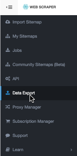
Data export menu
In the Amazon S3 tab, you’ll need to configure an S3 Sync by filling out your S3 key, secret, bucket, and region, then clicking connect:

Once connected, the green (Enabled) text confirms the sync is active. Beyond basic sync statistics, it shows us that a new file will appear in S3 for each scraping job. At this point, ensure your ‘File output format’ is JSON.

From your S3 console, you’ll see a new folder in your bucket called ‘web-scraper/’, within this folder you’ll see all your scraping jobs, and clicking into any one of these will show the JSON files associated with these jobs.

Finally, to successfully query from Athena, you’ll want to create a new folder to move a single JSON file which contains the data you want to use. When we create our Athena table, we point to a specific folder instead of a JSON file, so we want to ensure we isolate the JSON file in a corresponding folder.

Using Amazon Athena
You can complete the rest of the analysis entirely within Amazon Athena. To begin, you’ll need to navigate to the Query editor.
Creating a Table from an S3 Bucket
Unless you’re using a special Data Source setup, stick to using the default ‘AwsDataCatalog’. From the Tables and views tab, select Create and choose to create a table from S3 bucket data.

You’ll want to give your table a relevant name and will likely need to create a new database.

For your input data set, point to your S3 folder (not the JSON file):

You’ll need to specify your input file in JSON format and define your columns. The easiest way to accomplish this is to Bulk add columns:

Within the bulk add prompt, you’ll have to specify your columns and data types. Keep in mind that all values in the JSON object are data type string from the scraper, and we’ll perform conversion later.

After adding the columns, go ahead and click Create table. This will output and run a table generation query for you.

Querying the Data
To look at our table data and confirm it’s in a format we can use for our analysis, click the Preview Table button under the new table’s vertical ellipse menu.


Now we want to gather some useful information from this table. Remember, we wanted to know which states have the lowest prices for Ford Broncos. This is going to involve breaking down our query into a few steps:
- Changing our price string to a decimal data type
- Obtain an average of prices for each state
- Rank the average prices and filter for the lowest
Changing the Price Column to Decimal Data Type
Using our original preview query, we’ll instead need to select columns individually, so we can use the CAST() function to turn the price string into a decimal data type. We also had some Price columns with ‘Not Priced’, so we use a WHERE clause to filter these values out since they will not contribute to our average calculation later.
SELECT "seller-state",
       CAST(Price AS DECIMAL(10,2)) AS Price
FROM ford_bronco
WHERE Price != 'Not Priced'

Obtain an Average Price By State
We’ll GROUP BY state and perform an average calculation on the price to get an average price for each state.
SELECT "seller-state",
       AVG(CAST(Price AS DECIMAL(10,2))) as avg_price
FROM ford_bronco
WHERE Price != 'Not Priced'
GROUP BY "seller-state"

Ranking, Ordering, and Filtering Our Data
To make our solution generic for other datasets, we’re going to add a rank column for an ascending order of average prices:
SELECT "seller-state",
       AVG(CAST(Price AS DECIMAL(10,2))) as avg_price,
       RANK() OVER (ORDER BY AVG(CAST(Price AS DECIMAL(10,2))) ASC) rank
FROM ford_bronco
WHERE Price != 'Not Priced'
GROUP BY "seller-state"

At this point, we can already see ID is our cheapest state on average for a Ford Bronco. One of the huge benefits of using Amazon Athena with Web Scraper Cloud data is that running queries and looking at your results is a quick and simple process.
We’re going to finish out a generic solution which would work for a variety of datasets, but in many cases, you won’t need to go any further depending on what insights you need.
To filter for rank one, we use an outer query over our existing results to find the state and corresponding price with the first rank.
SELECT "seller-state", avg_price
FROM
    (SELECT "seller-state",
           AVG(CAST(Price AS DECIMAL(10,2))) as avg_price,
           RANK() OVER (ORDER BY AVG(CAST(Price AS DECIMAL(10,2))) ASC) rank
    FROM ford_bronco
    WHERE Price != 'Not Priced'
    GROUP BY "seller-state")
WHERE rank = 1

Summary
As you’ve seen here, Amazon Athena is a powerful tool for gathering insights from your Web Scraper Cloud jobs. However, there are several setup steps you’ll want to keep in mind to make this process a bit easier:
- Ensure you use the Web Scraper Cloud parser to format your data columns.
- Map your columns to AWS correctly.
- Ensure you’re looking at one JSON file by moving the target JSON into a new S3 Bucket folder.
In many cases, you’ll need to wrangle data by performing some type casting from string to other formats or removing blank or null values. After this wrangling, you’ve got all you need to interactively use Athena for gaining insights into your data.